We introduce two numerical algorithms to solve equations: the bissection algorithm and the Newton-Raphson algorithm. Newton-Raphson performs better, and we compare its implementations in a language that doesn't have Lisp style macros (Python) and one language that has them (Clojure), to illustrate what macros can do. On the way, the reader will have learned about numerical algorithms, symbolic derivation, some elements to write an interpreter, and the Lisp syntax.
So let's set ourselves to calculate $\sqrt{2}$. It is defined as the positive solution of $x^2=2$. Since the function $f:x\mapsto x^2$ is strictly increasing over $\mathbb{R}^+$, the equation $f(x)=2,x\geq 0$ has only one solution, and since $f(1)=1<2$ and $f(2)=4>2$, we know that this solution is between $1$ and $2$. We now calculate $f(1.5)=2.25>2$, so we have $1<\sqrt{2}<1.5$. We get a better approximation by calculating $f(\frac{1+1.5}{2})=f(1.25)=1.5625<2$ so we know that $1.25<\sqrt{2}<1.5$. We could carry on like that forever, but it will be faster to write a quick function to do that for us. Let's do it in Python:
def approx_sqrt_two(tol=0.00001,n_max=100):
    a,b = 1.0,2.0
    error = (b-a)/2
    n = 1
    while error > tol and n < n_max:
        candidate = (a+b)/2
        candidate_value = candidate**2
        if candidate_value > 2:
            b = candidate
        else:
            a = candidate
        n += 1
        error = (b-a)/2
    return candidate
The above code works well, but it can't be used to calculate any other things that $\sqrt{2}$. The first thing we can do is tweak it so it can calculate the square root of any number:
def approx_sqrt(target,tol=0.00001,n_max=100):
    a,b = 1.0,target
    error = (b-a)/2
    n = 1
    while error > tol and n < n_max:
        candidate = (a+b)/2
        candidate_value = candidate**2
        if candidate_value > target:
            b = candidate
        else:
            a = candidate
        n += 1
        error = (b-a)/2
    return candidate
So there it is, our new function approx_sqrt can calculate the
square root of any number. In fact we can do even better by enabling
our algorithm to be used for an arbitrary function.
What we want is to have a function with a signature :::python def
approx(func,target,tol=00001,n_max=100) where func will be a lambda
expression. Here is a first try:
def approx(func,target,a=0,b=100,tol=0.00001,n_max=100):
    error = (b-a)/2
    n = 1
    while error > tol:
        candidate = (a+b)/2
        candidate_value = func(candidate)
        if candidate_value > target:
            b = candidate
        else:
            a = candidate
        n += 1
        error = (b-a)/2
    return candidate
We now need to specify the bounds inside which the solution resides
(the arguments a and b), and also it assumes that func is
increasing (at the line if candidate_value > target:). If we assume
func is monotonic (either always increasing or always decreasing) we
can make a small modification to that code where we guess whether
func is increasing or decreasing, by calculating the rate
$\displaystyle\frac{\text{func}(b)-\text{func}(a)}{b-a}$:
def approx2(func,target,a=0,b=100,tol=0.00001,n_max=100):
    rate = (func(b)-func(a))/(b-a)
    compare = (lambda x,y: x > y) if rate > 0 else (lambda x,y: x < y)
    error = (b-a)/2
    n = 1
    while error > tol:
        candidate = (a+b)/2
        candidate_value = func(candidate)
        if compare(candidate_value, target):
            b = candidate
        else:
            a = candidate
        n += 1
        error = (b-a)/2
    return candidate
Let us go back to the first problem and see how fast the first algorithm performs to calculate $\sqrt{2}$. Is that algorithm efficient? We make a small change in the first version of the code to return how many iterations it required:
def approx_sqrt_two(f=lambda x:x**2,tol=0.00001,n_max=100):
a,b = 1.0,2.0
error = (b-a)/2
n = 1
while error > tol and n < n_max:
    candidate = (a+b)/2
    candidate_value = f(candidate)
    if candidate_value > 2:
        b = candidate
    else:
        a = candidate
    n += 1
    error = (b-a)/2
return candidate,n

:::Python
In [7]: approx_sqrt_two()
Out[7]: (1.4141998291015625, 17)
The code requires 17 iterations to calculate an approximation of $\sqrt{2}$ with a precision of 0.00001.
Can we do better? When searching for a better candidate that a and
b, the bisection algorithm takes the value
$\displaystyle\frac{a+b}{2}$. Taking the average is a reasonable
choice but it can seem a bit arbitrary, and that is where lies any
improvement of that algorithm. The algorithm of Newton-Raphson does
just that: it starts with $a$ as a first candidate, and then the
second candidate is calculated by solving:
$f'(a)(x-a)+f(a)=\text{target}$.
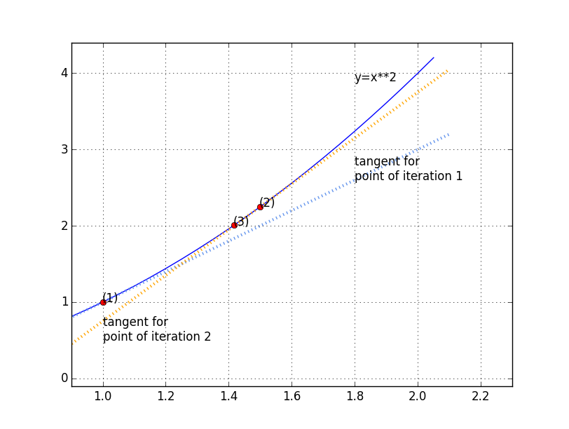
Why this formula? $y=f'(a)(x-a)+f(a)$ is the equation of the tangent in $a$ of the curve defined by $y=f(x)$.
The picture below the general principle: starts from point (1), draw the tangent of the curve there, find where the tangent intersects the like $y=2$, keep the corresponding abscissa and reiterate.
Here is the code for it:
def approx_sqrt_two_nr(tol=0.00001,n_max=100):
    a,b = 1.0,2.0
    n = 1
    candidate = a
    error = abs(candidate**2-2)
    while error > tol and n < n_max:
        candidate = (2-candidate**2)/(2.0*candidate) + candidate
        candidate_value = candidate**2
        n += 1
        error = abs(candidate**2-2)
    return candidate,n
The question that remains is: can we change the code to make it take a lambda argument like we did with the bisection algorithm?
Let us look as what it would take: the Newton-Raphson algorithm
requires to calculate the derivative of $f$, the function we want to
invert, which means taking a function (in our case: x**2) and
applying it a non trivial transformation (in our case it becomes2*x).
It is possible in any language to have a program that calculates symbolic derivatives. What is harder is to have this integrated with the rest of the code. Here is some pseudo code to implement Newton-Raphson in python with the function to solve as an input:
def approx_nr(func,target,candidate=0,tol=0.001,n_max=100):
    error = abs(func(candidate)-target)
    n = 1
    derivative_func = derivative(func) #this is the hard part
    while error > tol and n < n_max:
        candidate = (target-func(candidate))/derivative_func(candidate) + candidate
        candidate_value = func(candidate)
        n += 1
        error = abs(candidate_value-target)
    return candidate,n
Running that in the Python interpreter:
In [5]: approx_sqrt_two_nr()
Out[5]: (1.4142156862745099, 4)
It only takes 4 iterations against 17 iterations required by the bisection algorithm. Much faster!
The problem lies in the command derivative(func), which is supposed
to calculate the derivative of func. It is possible to do it with the
numerical derivative, which consists at approximating the quantity
$f'(x)$ with $f'(x) \simeq
\displaystyle\frac{f(x+\varepsilon)-f(x-\varepsilon)}{2\varepsilon}$
for a $\varepsilon$ small,
but I want to ignore this possibility as the goal of this article is
to discuss Lisp macros through symbolic derivative.
To calculate the symbolic derivative of a function, we need to have
first its expression, which isn't available with a lambda expression.
So we need to introduce a Function object that will contain that:
class Function:

    def __init__(self,expression,evaluation):
        self.expression = expression
        self.evaluation = evaluation
The question arises: how to store the function's expression? The
simplest answer, as a string (so x**2 would simply become "x**2")
turns out to be inconvenient to calculate the derivative. Instead it
is much better to store the expression as a direct representation of
the function syntactic tree:
   "**"
 /      \
"x" 2
This representation shows that the main function is "**" and its two
arguments are "x" and 2. One way to represent this
programmatically is to create a class like:
class NodeFunction:

    def __init__(self,main,arguments):
        self.main = main
        self.arguments = arguments
And our expression would become NodeFunction("**",["x",2]). If we
want to represent (x+1)**2 the same way, it would become:
NodeFunction("**",[NodeFunction("+",["x",1]),2]).
Another way is to represent our syntactic tree is through a list:
"x**2" becomes ["**","x",2], and "(x+1)**2" becomes
["**",["+","x",1],2].
Those two ways are equivalent but I will use the latter as it is more succinct, so I will stick with it for the rest.
We will need to be able to evaluate a syntactic tree at a given point.
For that we write a function whose signature will evaluate_tree(tree,values) where
values is going to be a dictionary (to allow multiple variables).
For example evaluate_tree(["+",1,"x"],{"x":2}) should read
["+",1,"x"], replace "x" by 2 when it encounters it, and proceed
the evaluation recursively. If tree is not a list, we will assume
it's either a number, in which case we return it, or a string, in
which case we assume that it is one of the keys of values, and
return its corresponding value.
If tree is a list, we take the main function that is tree[0] and the arguments. We
will evaluate the arguments using evaluate_tree recursively, and
once they are reduced to numbers we will be able to simply apply the
main function to them.
The code will be:
def evaluate_tree(tree,values):
    if type(tree) is not list:
        if type(tree) is str:
            return values[tree]
        else: #in that case we assume that tree is a number
            return tree
    main, args = tree[0], tree[1:]
    args_evaluated = map(lambda x: evaluate_tree(x,values),args)
    if main == "+":
        return sum(args_evaluated)
    if main == "-":
        return args_evaluated[0] - sum(args_evaluated[1:])
    if main == "*":
        #again,assuming only two arguments
        return args_evaluated[0]*args_evaluated[1]
    if main == "/":
        return args_evaluated[0]/args_evaluated[1]
    if main == "**":
        return args_evaluated[0]**args_evaluated[1]
    #for the rest of the function, we assume only one argument
    #the functions log, exp, cos and sin need to be imported
    #from the math module
    if main == "ln":
        return log(args_evaluated[0])
    if main == "exp":
        return log(args_evaluated[0])
    if main == "cos":
        return cos(args_evaluated[0])
    if main == "sin":
        return sin(args_evaluated[0])
    return None
This is not the most robust code, but it will fit for illustrative purpose.
Let's calculate the derivative of a function! Before that, here is a reminder of the rules to calculate the derivative:
$\frac{d(f+g)}{dx} = \frac{df}{dx}+\frac{dg}{dx}$
$\frac{d(f-g)}{dx} = \frac{df}{dx} - \frac{dg}{dx}$
$\frac{d(fg)}{dx} = \frac{df}{dx}g + f\frac{dg}{dx}$
$\frac{d(f/g)}{dx} = \frac{\frac{df}{dx}g-f\frac{dg}{dx}}{\big(\frac{dg}{dx}\big)^2}$
$\frac{d(f(g))}{dx} = \frac{dg}{dx}\Big(\frac{df}{dx}\Big)(g)$
And the derivatives of elementary functions:
$\frac{dx}{dx} = 1$
$\frac{dK}{dx} = 0$ If $K$ is a constant (with respect to $x$).
$\frac{dx^n}{dx} = nx^{n-1}$
$\frac{d(\cos x)}{dx} = -\sin x$
$\frac{d(\sin x)}{dx} = \cos x$
$\frac{de^x}{dx} = e^x$
$\frac{d\ln x}{dx} = \frac{1}{x}$
Let's now write a function that calculates the symbolic derivative of a mathematical expression. We will restrict ourselves to the functions listed above.
The our function will take a mathematical expression as an argument,
along with the variable we are calculative the derivative with respect
to. So the signature of our function will be
derivative(expr,variable).
The mechanism to calculate the symbolic derivative of a syntactic tree is very similar to the mechanism to evaluate a syntactic tree: we go down the tree, if the tree is a constant or a variable, calculating the derivative is straightforward (it's $1$ if the expression is equal to the variable, and $0$ otherwise). So the start of the function will look like:
def derivative(expr,variable):
    if type(expr) is not list:
        return 1 if expr == variable else 0
    main, args = expr[0],expr[1:]
    ...
If the tree is a list, the code will break down the expression into the main
function (the first element of the list) and its arguments (the rest
of the list).
Then we will check what is the value of main and apply the
corresponding formula to the arguments. For example, if main is
"+", it will look like:
derivative_args = map(lambda x:derivative(x,variable),args)
return ["+"]+derivative_args
For the other possible values of main we will apply the rules of the
derivation that we saw above.
At the end the whole function is:
def derivative(expr,variable):
    if type(expr) is not list:
        return 1 if expr == variable else 0
    main, args = expr[0], expr[1:]
    if main == "+":
        derivative_args = map(lambda x:derivative(x,variable),args)
        return ["+"]+derivative_args
    if main == "*":
        u,v = args[0],args[1] #assume there are only two arguments
        du, dv = derivative(u,variable), derivative(v, variable)
        return ["+",["*",du,v],[u,dv]]
    if main == "/":
        u,v = args[0],args[1] #assume there are only two arguments
        du, dv = derivative(u,variable), derivative(v, variable)
        return ["/",["-",["*",du,v],["*",u,dv]],["**",v,2]]
    if main == "**":
        u,v = args[0],args[1] #assume there are only two arguments
        du, dv = derivative(u,variable), derivative(v, variable)
        return ["*",["+",dv,["/",du,u]],["**",u,v]]
    if main == "exp": #exponential function
        u = arg[0] #assume one argument only
        du = derivative(u,variable)
        return ["*",du,["exp",u]]
    if main == "ln":
        u = arg[0] #assume one argument only
        du = derivative(u,variable)
        return ["/",du,u]
    if main == "cos":
        u = arg[0] #assume one argument only
        du = derivative(u,variable)
        return ["*",du,["*",-1,["sin",u]]]
    if main == "sin":
        u = arg[0] #assume one argument only
        du = derivative(u,variable)
        return ["*",du,["cos",u]]
    return None
Again, this is not the most robust code and has some defaults (for example, the multiplication can only take two arguments) but it is simple and illustrates how symbolic derivatives are calculated.
What remains is now to integrate the derivative function with the
rest of the code. It requires a small modification of the prototype
code we wrote in a previous paragraph (func is gonna be a Function
object that was described above):
def approx_nr(func,target,candidate=0,tol=0.001,n_max=100):
    error = abs(func(candidate)-target)
    n = 1
    derivative_func = derivative(func.expression)
    while error > tol and n < n_max:
        candidate = (target-func(candidate))/evaluate_tree(derivative_func,{"x":candidate}) + candidate
        candidate_value = func(candidate)
        n += 1
        error = abs(candidate_value-target)
    return candidate,n
The Lisp syntax is different of most language: instead of having
function(arg1,arg2), lisp is (function arg1 arg2). The operators
don't have a special syntax, so for example 1+2*(3-4) is (+ 1 (* 2
(- 3 4))). Please notice that it is very similar to how we expressed
the syntactic tree earlier.
Since the rest of the code in the article is going to be in Clojure, I will give a brief overview of the Clojure language. Feel free to skip if you're already familiar with this language.
Global variables are defined using def. For example:
user=> (def x 4)
#'user/x
user=> x
4
Local variables are defined using let. For example:
user=> (let [x 5]
#_=>    (* 2 x))
10
Inside this let is defined the variable x equal to 5. We then
calculate (* 2 x).
let's can be used to define multiple variables at the same time,
some depending of the previous ones:
user=> (let [x 1
#_=>       y 2
#_=>       z (+ x y)]
#_=>   (* 2 z))
6
Clojure can also take anonymous functions, they can be expressed in
two ways: #(+ 1 %) (% is the argument, if there are multiple
arguments it becomes #(+ 1 %1 %2)), or using fn: (fn [x] (+ 1
x)).
Anonymous functions are called just like standard functions, except that instead of their names, it's their full codes that is given:
user=> ((fn [x] (+ 1 x)) 5)
6
A function is created using defn. For example:
(defn my-function [x]
    (+ 1 x))
defn can also be used to define several times the function with
different arguments:
(defn my-other-function [x]
        (my-other-function [x 2])
      my-other-function [x y]
        (* x y))
That was my-other-function can take either one or two arguments.
It is also possible to use def to define a function:
(def yet-another-function (fn [x]
    (+ 2 x)))
In Clojure, vectors are between brackets: [1, 2, 3] and lists are
between parenthesis, but they are quoted so they are not evaluated:
'(1 2 3). The function to get an element of a list is nth:
user=> (nth '(1 2 3 4 5 6) 2)
3
It is very common to want to access to the first element of a list,
and also to the rest of the elements of that list. For that two
functions exist: first and rest:
user=> (first '(1 2 3 4))
1
user=> (rest '(1 2 3 4))
(2 3 4)
Clojure data are immutable, so lists can't be modified. However, it is
possible to construct a new list from a list and a new element, where
the new element is put at the beginning of the new list, with the function
cons:
user=> (cons 0 '(1 2 3))
(0 1 2 3)
Like in most of the programming languages, Clojure has if
conditions, that takes a boolean, a value to return if the boolean is
true and another value to return otherwise.
user=> (if (> 3 4) 1 2)
2
There is also a switch statement called cond to test several
conditions on data. cond has to contain a default case, named
`:default':
user=> (defn show-cond [x]
#_=>      (cond (< x 0) "negative"
#_=>            (< x 10) "small"
#_=>            (< x 100) "normal"
#_=>            (< x 1000) "big"
#_=>            :default "really big"))
#'user/show-cond
user=> (show-cond 100000)
"really big"
user=> (show-cond -1)
"negative"
user=> (show-cond 5)
"small"
For performance issues, recursions are done with recur.
(defn my-sum [a-list]
         (my-sum a-list 0)
      my-sum [a-list pre-sum]
         (if (nil? a-list) 0
             (let [x (first a-list)
                   xs (rest a-list)]
               (recur xs (+ pre-sum x)))))
Loops also work with recur, here is an example
(defn my-other-sum [a-list]
    (loop [res 0
           lst a-list]
       (if (nil? lst) res
           (let [x (first a-list)
                 xs (rest a-list)]
             (recur (+ res x) xs)))))
Macros can be seen as special functions that enable the programmer to modify the syntax of the language. How? By controlling how the arguments are getting evaluated. Is that an helpful explanation? Probably not but I hope to be able to shed some light soon by giving an example of a concrete macro.
The python code above for Newton-Raphson can easily be translated into Clojure.
First, the derivative:
(defn derivative [function variable]
    (if (not (seq function)) (if (= function variable) 1 0)
        (let [main (first function)
              args (rest function)
              der (fn [x] (derivative x variable))]
          (cond
            (= '+ main) (cons '+ (map der args))
            (= '- main) (cons '- (map der args))
            (= '* main) (let [u (nth args 0)
                              du (der u)
                              v (nth args 1)
                              dv (der v)]
                          (list '+ (list '* u dv) (list '* v du)))
            (= '/ main) (let [u (nth args 0)
                              du (der u)
                              v (nth args 1)
                              dv (der v)]
                          (list '/ (list '- (list '* du v) (list
'* u dv)) (list '** v 2)))
            (= '** main) (let [u (nth args 0)
                               du (der u)
                               v (nth args 1)
                               dv (der v)]
                           (list '_ (list '+ dv (list '/ du u)
(list '** u v))))
            (= 'exp main) (let [u (nth args 0)
                                du (der u)]
                            (list '* du (exp u)))
            (= 'ln main) (let [u (nth args 0)
                                du (der u)]
                            (list '/ du u))
            (= 'cos main) (let [u (nth args 0)
                                du (der u)]
                            (list '* ('* -1 du) (list 'sin u)))
            (= 'sin main) (let [u (nth args 0)
                                du (der u)]
                            (list '* du (list 'sin u)))
            :default nil))))
We can then do exactly the same as in Python and write a function
approx-nr whose signature will be (defn approx-nr
[function syntactic-tree target tolerance min-val max-val]) that will be
called like: (approx-nr (fn [x] (** x 2)) '(** 2 x) 2 0.00001 1 2).
But since the two arguments function and syntactic-tree are very
closed (syntactic-tree is, after all, the syntactic tree of
function, and with the Lisp syntax the code of a function is its
syntactic tree...) it is a legitimate concern to want to avoid using
an extra argument and get the syntactic tree directly from function.
For that, we would have to tell the compiler something in the line of
"Hey, do not evaluate
[I don't know if the best term for that is 'evaluate' or 'byte compile'
or 'interpret'] function directly, but before that give me its
source code so I can calculate its derivative!" This is not possible
with a standard function - we don't have control when arguments are
evaluated, but with a macro, it is: here is a macro that extracts the
source code of an anonymous function: (defmacro get-code [func] (list
'quote (nth func 2)))
First let's see how it works in the Clojure interpreter:
user=> (get-code (fn [x] (+ 1 x)))
(+ 1 x)
How did that work? when calling get-code, func is replaced by the
value we gave it, in our case (fn [x] (+ 1 x)), but it is not
evaluated. That is not the case with functions, so a language like
Python that doesn't have macros can't do that. Then, (fn [x] (+ 1
x)) is treated as a normal list, so (nth func 2) returns the 3rd
value in that list, in our case (+ 1 x). The quote in get-code
is here to say "ok, treat that as a list instead of trying to evaluate
it". The symbol ' before the quote is here to tell the clojure
compiler not to eval quote right away.
We can see how the get-code macro is expanded, using macroexpand:
user=> (macroexpand '(get-code (fn [x] (+ 1 x))))
(quote (+ 1 x))
Then that last line (quote (+ 1 x)) is evaluated and at the end it
returns the list (+ 1 x).
Once we have extracted the code of func we will calculate its
derivative as a list representing its syntactic tree, and then we will
need to make a function out of it. This can be done with a macro:
(defmacro make-function [variable core]
    (list 'fn [variable] core))
We can get the variables names of a function the same way we got its
code. For the sake of conciseness I gonna assume the functions here only
have one variable, so the code to get that variable name is: (defmacro get-variable [func] (list 'quote (nth (nth func 1) 0))).
Armed with those two utility macros and the derivative function we
are able to write the code for the Newton-Raphson algorithm:
(defn approx-nr
    ([func target] (approx-nr func target start 0.00000001 100))
    ([func target start tolerance n-iterations]
        (let [variable (get-variable func)
              code (get-code func)
              der (make-function (derivative code variable))]
          (loop [k 0
                 res start]
              (if (or
                     (>= k n-iterations)
                     (< (Math/abs (- (func res) target)) tolerance))
                 res
                 (recur (inc k) (+ res (/ (- target (func res)) (der res)))))))))
The main difference with the Python version is that we don't need to
pass the syntactic tree of func to our algorithm since it is
extracted directly from func's code.
The python version of the Newton-Raphson algorithm required to
implement a function eval_tree that can evaluate a syntactic tree,
which is basically a small subset of a Lisp interpreter. The Lisp
version doesn't need that, which makes the code shorter as a result,
and also safer as it is not possible to pass to the Newton-Raphson
algorithm a wrong syntactic tree for the function we are trying to solve.
Instead, we have embedded in our code a very small Computer Algebra System that operates directly on the code we use. This would not have been possible without macros. The Lisp guru and evangelist Paul Graham wrote: "It would be convenient here if I could give an example of a powerful macro, and say there! how about that? But if I did, it would just look like gibberish to someone who didn't know Lisp; there isn't room here to explain everything you'd need to know to understand what it meant. In Ansi Common Lisp I tried to move things along as fast as I could, and even so I didn't get to macros until page 160." [0] Here we managed to give an example of a powerful macro in much less than 160 pages.
However, the goal for which we had use of macros, numerically solving arbitrary equations, isn't the most common task in programming, and I believe this is for this reasons we had to use a macro: if it was something people did a lot, the functionalities to calculate derivatives of anonymous functions would have been incorporated to popular languages.
Thus macros are useful for greenfield projects, and once such projects become mainstream functionalities provided by macros get put into mainstream languages.
Python specifically has two modules that can be used: the Python
parser ast and the inspect module to be able to get the source
code of a function as a string.
In [7]: inspect.getsource(lambda x: 2*x)
Out[7]: u'inspect.getsource(lambda x: 2*x)\n'
It is thus possible to have a function that takes a lambda expression
as an argument, get its source code through inspect and parses it
with ast to get the syntactic tree, then calculate the derivative of
that tree and make a lambda expression out of it.
However this approach is very specific to Python, which is why it wasn't much discussed here: I used Python to represent languages that don't have macros, and this approach would not be doable in Java for example.
[0] http://paulgraham.com/avg.html